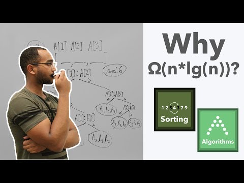
The Comparison Decision-Tree Model
In the comparison model of computation, elements are treated as abstract black boxes: an algorithm may copy or swap elements, but the only way it can inspect key values is by executing a binary comparison $a_i : a_j$ (returning $<, =, >$, or for distinct keys, simply $a_i < a_j$ vs. $a_i > a_j$). Operations like bit extraction, array indexing by key value ($C[A[i]]$), or hashing key bytes are disallowed.
Any comparison sort on an input of fixed size $n$ can be unrolled into a finite binary decision tree $T_n$:
- Each internal node is labeled by a pair of indices $(i : j)$ and branches left if $A[i] < A[j]$ or right if $A[i] > A[j]$.
- Each leaf is labeled by a permutation $\pi = (\pi(1), \pi(2), \dots, \pi(n)) \in S_n$ that reorders the input into sorted order $A[\pi(1)] < A[\pi(2)] < \dots < A[\pi(n)]$.
- The worst-case number of comparisons on inputs of size $n$ equals the height $h(T_n)$ (longest root-to-leaf path).
- The average-case number of comparisons over a uniform distribution of all $n!$ permutations equals the average leaf depth $\frac{\text{IPL}(T_n)}{n!}$.
Step 1 (Injectivity of Leaves): Suppose two distinct input permutations $\sigma_1 \ne \sigma_2 \in S_n$ follow the exact same sequence of comparison outcomes from the root to the same leaf $\ell$. Then the algorithm applies the exact same output permutation $\pi$ to both $\sigma_1$ and $\sigma_2$. Since $\sigma_1 \ne \sigma_2$, at least one of $\pi(\sigma_1)$ or $\pi(\sigma_2)$ fails to be sorted! Hence every one of the $n!$ permutations must reach a distinct leaf, so the number of reachable leaves $L$ satisfies $L \ge n!$.
Step 2 (Binary Tree Capacity): A binary tree of height $h$ has at most $2^h$ leaves ($L \le 2^h$). Combining both inequalities gives $2^h \ge L \ge n!$, or:
$$h \ge \lceil \log_2(n!) \rceil$$Step 3 (Stirling's Approximation): Using Stirling's lower bound $n! = \sqrt{2\pi n}\left(\frac{n}{e}\right)^n e^{\theta_n}$ (where $\frac{1}{12n+1} < \theta_n < \frac{1}{12n}$), or equivalently bounding the sum $\ln(n!) = \sum_{k=1}^n \ln k \ge \int_1^n \ln x\,dx = n \ln n - n + 1$:
$$\log_2(n!) = n \log_2 n - \frac{n}{\ln 2} + \frac{1}{2}\log_2(2\pi n) + O\!\left(\frac{1}{n}\right) \approx n \log_2 n - 1.4427\,n + \frac{1}{2}\log_2(2\pi n)$$Step 4 (Average-Case & Randomized Lower Bound): By convexity of $f(d) = 2^d$ (or Kraft's inequality), among all binary trees with $L \ge n!$ leaves, the sum of leaf depths $\sum_{\ell=1}^{L} d(\ell)$ is minimized when the tree is almost complete (all leaves at depth $\lfloor \log_2 L \rfloor$ or $\lceil \log_2 L \rceil$), yielding average leaf depth $\ge \log_2(n!) - 1 = n \log_2 n - O(n)$. By Yao's Minimax Principle, any randomized comparison sort also requires $\ge \log_2(n!) - O(1)$ expected comparisons!
Step through Bentley-McIlroy 3-way partition QuickSort, Bottom-Up MergeSort inversion counting, and non-comparison LSD RadixSort with live comparison and swap counters.
Invariant & State
| Problem / Input Constraint | Reachable States $L$ | Comparison Lower Bound $\lceil \log_2 L \rceil$ | Optimal Matching Algorithm |
|---|---|---|---|
| General Sorting ($n$ distinct keys) | $n!$ | $n \log_2 n - 1.443n + \Theta(\log n)$ | Ford-Johnson Merge-Insertion / Merge Sort |
| Multiset Sorting ($f_1, \dots, f_k$ duplicates) | $\frac{n!}{f_1! f_2! \cdots f_k!}$ | $n H(p_1, \dots, p_k) - O(k \log n)$ | Bentley-McIlroy / Dijkstra 3-Way Quicksort |
| $k$-Nearly Sorted ($|i - \pi(i)| \le k$) | $\le (2k + 1)^n$ | $\Omega(n \log k)$ | Min-Heap Sliding Window ($O(n \log k)$) |
| Inversion-Bounded ($I(A) \le I$) | $\le \binom{n + I}{I}$ | $\Omega\!\left(n \log\!\left(1 + \frac{I}{n}\right)\right)$ | Finger Search Tree / Adaptive TimSort |
Exact Minimum Comparisons for Small $N$ & Adversary Arguments
How close is $\lceil \log_2(n!) \rceil$ to the true minimum worst-case comparisons $S(n)$? For $n = 1 \dots 11$, Ford and Johnson's Merge-Insertion Sort (1959) matches $\lceil \log_2(n!) \rceil$ to the exact single comparison:
- $n = 3$: $\lceil \log_2 6 \rceil = 3$ comparisons.
- $n = 4$: $\lceil \log_2 24 \rceil = 5$ comparisons.
- $n = 5$: $\lceil \log_2 120 \rceil = 7$ comparisons! (Whereas standard Merge Sort and Insertion Sort take $8$ or $10$ comparisons; sorting $5$ elements in $7$ comparisons requires pairing $(a,b)$ and $(c,d)$, comparing their winners, and binary-inserting $e$ and the loser along a 3-element chain).
- $n = 12$: $\lceil \log_2(12!) \rceil = 29$, but Wells (1965) proved by exhaustive computer search that $S(12) = 30$, showing that no comparison tree can split $12!$ into perfectly balanced $50/50$ subsets at every step!
min/maxOn modern CPUs, performing 7 heavily branched comparisons to sort 5 integers is actually slower than executing 9 branchless conditional-move (CMOV) or SIMD (_mm_min_epi32 / _mm_max_epi32) compare-and-swap operations in a Sorting Network (Batcher's Odd-Even Merge or optimal 5-element / 8-element Bose-Nelson networks). Because all comparator wires in a sorting network layer are data-independent, a superscalar CPU executes 3–4 compare-and-swaps in a single clock cycle with zero branch mispredictions!
Production C++20 Implementation: Optimal 7-Comparison 5-Sort vs. Branchless Sorting Network
#include <array>
#include <cmath>
#include <concepts>
#include <cstdint>
#include <utility>

// Information-theoretic lower bound ceil(log2(n!)) using exact log-gamma / sum of log2(k)
inline std::uint64_t comparison_lower_bound(std::uint64_t n) noexcept {
    double log2_fact = 0.0;
    for (std::uint64_t k = 2; k <= n; ++k) {
        log2_fact += std::log2(static_cast<double>(k));
    }
    return static_cast<std::uint64_t>(std::ceil(log2_fact - 1e-12));
}

// Ford-Johnson Merge-Insertion Sort for N = 5 in AT MOST 7 Comparisons (Optimal!)
template <std::totally_ordered T>
std::array<T, 5> sort5_optimal_7cmps(T a, T b, T c, T d, T e) noexcept {
    if (b < a) std::swap(a, b); // Cmp 1: a <= b
    if (d < c) std::swap(c, d); // Cmp 2: c <= d
    if (d < b) {                // Cmp 3: order pairs by larger element (b <= d)
        std::swap(a, c);
        std::swap(b, d);
    }
    // Now we have main chain: a <= b <= d, and c <= d.
    // Step 4-5: Binary insert e into the 3-element chain [a, b, d] (2 comparisons)
    std::array<T, 4> chain;
    if (e < b) {                // Cmp 4
        if (e < a) chain = {e, a, b, d}; // Cmp 5a
        else       chain = {a, e, b, d};
    } else {
        if (e < d) chain = {a, b, e, d}; // Cmp 5b
        else       chain = {a, b, d, e};
    }
    // Step 6-7: Since c <= d, c is smaller than d (which is at chain[2] or chain[3]),
    // so c only needs to be binary-inserted into the first 3 elements chain[0..2] (2 comparisons)!
    if (c < chain[1]) {         // Cmp 6
        if (c < chain[0]) return {c, chain[0], chain[1], chain[2], chain[3]}; // Cmp 7a
        else              return {chain[0], c, chain[1], chain[2], chain[3]};
    } else {
        if (c < chain[2]) return {chain[0], chain[1], c, chain[2], chain[3]}; // Cmp 7b
        else              return {chain[0], chain[1], chain[2], c, chain[3]};
    }
}

// Contrast: Branchless 9-Comparator Sorting Network for N = 5 (Compiles to CMOV / min-max)
template <std::totally_ordered T>
void sort5_branchless_network(T* v) noexcept {
    auto cmp_swap = [](T& x, T& y) noexcept {
        T mn = (y < x) ? y : x;
        T mx = (y < x) ? x : y;
        x = mn; y = mx;
    };
    cmp_swap(v[0], v[1]); cmp_swap(v[3], v[4]);
    cmp_swap(v[2], v[4]); cmp_swap(v[2], v[3]);
    cmp_swap(v[0], v[3]); cmp_swap(v[0], v[2]);
    cmp_swap(v[1], v[4]); cmp_swap(v[1], v[3]);
    cmp_swap(v[1], v[2]);
}Whenever an interview or systems design problem asks you to sort in $o(N \log N)$ time, ask: Which assumption of the comparison decision-tree model can we violate?
1. Non-Comparison Multi-Way Branching: Counting Sort and Radix Sort use key digits as direct array indices ($b$-way branching per step instead of $2$-way), yielding height $\log_b(n!)$.
2. Restricted Input Space ($L \ll n!$): If the array has at most $O(n)$ inversions or comes from merging $O(1)$ sorted streams, there are only $2^{O(n)}$ valid inputs, so an adaptive comparison sort finishes in $\Theta(n)$ comparisons!