Mergeable Priority Queues: Leftist, Skew, Binomial & Fibonacci Heaps (O(1) Decrease-Key)

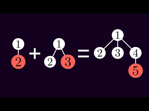
From Leftist/Skew Spine Merging to Binomial & Fibonacci Forests

Let us compare the four classical mergeable priority queue families:

1. Leftist Heap (Crane 1972) & Skew Heap (Sleator & Tarjan 1986): A Leftist Heap stores the null-path length $\text{npl}(u)$ (shortest distance to a null child) at each node and enforces $\text{npl}(u.\text{left}) \ge \text{npl}(u.\text{right})$. Consequently, the right spine has length at most $\lfloor \log_2(N + 1) \rfloor$. Merging two Leftist Heaps recursively merges their right spines in $O(\log N)$ worst-case time and swaps children where needed. A Skew Heap drops the stored $\text{npl}$ field entirely and unconditionally swaps left and right children at every node along the merged right spine, achieving $O(\log N)$ amortized time!
2. Binomial Heap (Vuillemin 1978): A Binomial Tree $B_k$ of order $k$ has $2^k$ nodes and is formed by linking two $B_{k-1}$ trees (attaching one as the leftmost child of the other's root). Any integer $N = \sum b_k 2^k$ decomposes uniquely into at most $\lfloor \log_2 N \rfloor + 1$ Binomial Trees, so meld(H₁, H₂) is literally ripple-carry binary addition on tree orders in $O(\log N)$ time.
3. Fibonacci Heap (Fredman & Tarjan 1987): Relaxes the Binomial Heap by allowing multiple trees of the same degree in a circular doubly-linked root list during insert and meld ($O(1)$ actual time), only consolidating trees of equal degree by array-indexed bucket linking during extractMin.
4. Pairing Heap (Fredman, Sedgewick, Sleator & Tarjan 1986): A self-adjusting multi-ary tree where extractMin links root children in adjacent pairs left-to-right and then coalesces right-to-left. Achieves $O(1)$ insert/meld, $O(\log N)$ extractMin, and $o(\log N)$ ($Omega(\log \log N)$) amortized decreaseKey with a fraction of the pointer overhead of Fibonacci Heaps.

Visualizing Fibonacci Heap Cascading Cuts & Degree-Table Consolidation

Implementation: Skew Heap $O(\log N)$ Amortized Meld in 12 Lines of C++

When you genuinely need a pointer-based mergeable priority queue in production or competitive programming, the Skew Heap provides $O(\log N)$ amortized meld, push, and pop in just a dozen lines of code with zero balance metadata fields:

// C++20: Skew Heap — Self-Adjusting Mergeable Priority Queue in O(log N) Amortized Time
#include <utility>

struct SkewNode {
    int key;
    SkewNode *left = nullptr, *right = nullptr;
    explicit SkewNode(int k) : key(k) {}
};

// Merges two Skew Heaps in O(log N) amortized time by unconditionally swapping children
SkewNode* meld(SkewNode* a, SkewNode* b) {
    if (!a) return b;
    if (!b) return a;
    if (b->key < a->key) std::swap(a, b);
    // Recursively merge b with a's right spine, then swap a's children
    a->right = meld(a->right, b);
    std::swap(a->left, a->right);
    return a;
}

SkewNode* push(SkewNode* root, int key) {
    return meld(root, new SkewNode(key));
}

SkewNode* popMin(SkewNode* root) {
    SkewNode* nextRoot = meld(root->left, root->right);
    delete root;
    return nextRoot;
}