1. Formal Invariant — Quadrangle Inequality + Interval Monotonicity
Invariant: Knuth-Yao Interval Split Monotonicity
Consider the interval recurrence for $1 \le i \le j \le N$:
$$dp[i][j] = C(i, j) + \min_{i \le k < j} \Big( dp[i][k] + dp[k+1][j] \Big)$$
Suppose the cost function $C(i, j)$ satisfies two conditions for all $a \le b \le c \le d$:
- Quadrangle Inequality (QI): $C(a, c) + C(b, d) \le C(a, d) + C(b, c)$
- Interval Containment Monotonicity: $C(b, c) \le C(a, d)$ whenever $[b, c] \subseteq [a, d]$
Then the optimal split point $opt[i][j] = \arg\min_{k} (dp[i][k] + dp[k+1][j])$ satisfies:
$$opt[i][j-1] \le opt[i][j] \le opt[i+1][j]$$
When iterating in increasing order of interval length $L = j - i$, both $opt[i][j-1]$ and $opt[i+1][j]$ are already known from length $L - 1$, bounding the inner loop for $k$ to $[opt[i][j-1],\; opt[i+1][j]]$.
Why does this reduce the total time to $O(N^2)$? Fix an interval length $L$ and sum the number of candidate split points $k$ tested across all $i \in [1, N - L]$:
$$\sum_{i=1}^{N-L} \Big( opt[i+1][i+L] - opt[i][i+L-1] + 1 \Big)$$
Notice that the term $opt[i+1][i+L]$ for index $i$ cancels against $-opt[(i+1)][(i+1)+L-1]$ at index $i+1$! It is a telescoping sum bounded by $(opt[N-L+1][N] - opt[1][L]) + N \le 2N$. Summing $O(N)$ work across $N$ lengths gives $O(N^2)$ total operations.
2. Telescoping Interval Search Topology
Known split: opt[i][j-1]"] RightSub["Interval [i+1, j]
Known split: opt[i+1][j]"] end subgraph LengthL["Current Target (Length L)"] Target["Interval [i, j]
Search only k in [opt[i][j-1], opt[i+1][j]]"] end LeftSub -->|Lower Bound| Target RightSub -->|Upper Bound| Target
3. Canonical Applications: Optimal BST & Optimal Matrix / File Merging
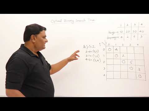
- Optimal Binary Search Tree (Knuth 1971): Given sorted keys $K_1 < K_2 < \dots < K_N$ with access probabilities $p_1, \dots, p_N$, placing root $K_k$ pushes both subtrees one level deeper, adding $C(i, j) = \sum_{m=i}^{j} p_m$ to the expected search cost. Because $C(i, j)$ is an additive interval sum, $C(a, c) + C(b, d) = C(a, d) + C(b, c)$ (QI holds with equality!) and $C(b, c) \le C(a, d)$ for $p_m \ge 0$.
- Optimal Alphabetic Merge / Stone Merging: Merging adjacent piles $i \dots j$ into one pile costs the sum of weights $W(i, j) = \text{pref}[j] - \text{pref}[i-1]$. Again QI holds with equality, so Knuth's Optimization solves adjacent stone merging in $O(N^2)$ (and the Garsia-Wachs algorithm further reduces this specific case to $O(N \log N)$).
4. Hardware & Memory Access Reality
Row-Major vs Diagonal Traversal Cache Layout
In naive interval DP looped by length $L$, dp[i][k] reads across row i (contiguous in row-major order), while dp[k+1][j] reads down column j (stride $N$). However, because Knuth's Optimization restricts $k$ to an average of 1 to 2 iterations per state, the inner loop finishes almost instantaneously inside L1 cache! Equivalently, iterating i downwards from $N$ to $1$ and j upwards from $i+1$ to $N$ computes both dependencies $(i, j-1)$ and $(i+1, j)$ in pure row-order without needing an outer length loop.
5. Complexity Matrix
Inspect how Quadrangle Inequality C(a,c)+C(b,d) ≤ C(a,d)+C(b,c) forces decision monotonicity opt[i][j-1] ≤ opt[i][j] ≤ opt[i+1][j], collapsing O(N³) transitions.
Invariant & State
| Algorithm / Variant | Time Complexity | Space Complexity | Conditions Required |
|---|---|---|---|
| Naive Interval DP (Optimal BST / Merge) | O(N^3) | O(N^2) | Any interval cost $C(i, j)$ |
| Knuth-Yao Interval Optimization | O(N^2) | O(N^2) | QI + Interval Monotonicity on $C(i, j)$ |
| Garsia-Wachs (Order-Preserving Merge Only) | O(N log N) | O(N) | Additive $C(i, j) = \sum_{m=i}^j w_m$ |
6. Production-Grade C++20 Implementation
#include <vector>
#include <cstdint>
#include <limits>

struct KnuthResult {
    int64_t min_cost;
    std::vector<std::vector<int>> opt;
};

// Solves min-cost adjacent stone merge / Optimal BST in O(N^2) time
KnuthResult solve_knuth_interval_dp(const std::vector<int64_t>& weights) {
    const int n = static_cast<int>(weights.size());
    constexpr int64_t INF = std::numeric_limits<int64_t>::max() / 4;

    std::vector<int64_t> pref(n + 1, 0);
    for (int i = 0; i < n; ++i) pref[i + 1] = pref[i] + weights[i];
    auto cost = [&](int i, int j) -> int64_t {
        return pref[j + 1] - pref[i];
    };

    std::vector<std::vector<int64_t>> dp(n, std::vector<int64_t>(n, INF));
    std::vector<std::vector<int>> opt(n, std::vector<int>(n, 0));

    for (int i = 0; i < n; ++i) {
        dp[i][i] = 0;
        opt[i][i] = i;
    }

    // Iterate i downwards and j upwards so (i, j-1) and (i+1, j) are ready
    for (int i = n - 2; i >= 0; --i) {
        for (int j = i + 1; j < n; ++j) {
            int64_t best = INF;
            int best_k = opt[i][j - 1];
            int upper_k = std::min(j - 1, opt[i + 1][j]);

            for (int k = opt[i][j - 1]; k <= upper_k; ++k) {
                int64_t cand = dp[i][k] + dp[k + 1][j] + cost(i, j);
                if (cand < best) {
                    best = cand;
                    best_k = k;
                }
            }
            dp[i][j] = best;
            opt[i][j] = best_k;
        }
    }
    return {dp[0][n - 1], opt};
}
Production Pitfall — Why Matrix Chain Multiplication Does NOT Satisfy Knuth's Optimization
In Matrix Chain Multiplication, merging $A_{i..k}$ (dimensions $p_i \times p_{k+1}$) with $A_{k+1..j}$ (dimensions $p_{k+1} \times p_{j+1}$) costs $p_i \cdot p_{k+1} \cdot p_{j+1}$. Notice that this merge cost depends on the split point $k$ itself, not just the outer endpoints $(i, j)$, and does not obey interval monotonicity! Applying Knuth's Optimization to Matrix Chain Multiplication produces wrong answers (use the Hu-Shing $O(N \log N)$ polygon triangulation algorithm instead).