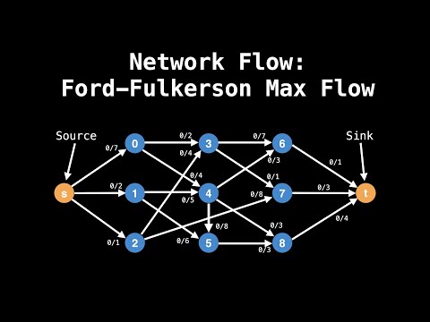
Formal Flow Network Invariants & The Residual Graph $G_f$
A flow network $G = (V, E, c, s, t)$ is a directed graph with source $s \in V$, sink $t \in V$, and capacity function $c: V \times V \to \mathbb{R}_{\ge 0}$. An $s$-$t$ flow is a function $f: V \times V \to \mathbb{R}$ satisfying three axioms:
- Capacity Constraint: For all $u, v \in V$, $0 \le f(u, v) \le c(u, v)$.
- Flow Conservation: For every internal node $u \in V \setminus \{s, t\}$, total incoming flow equals total outgoing flow: $$\sum_{v \in V} f(v, u) = \sum_{w \in V} f(u, w)$$
- Residual Capacity $c_f(u, v)$: Given flow $f$, the residual network $G_f = (V, E_f)$ contains all edges with strictly positive residual capacity $c_f(u, v) > 0$, defined for each directed edge $(u, v) \in E$ as: $$c_f(u, v) = c(u, v) - f(u, v) \quad (\text{forward unused capacity})$$ $$c_f(v, u) = f(u, v) \quad (\text{backward undo capacity})$$
Why Backward Edges Are Essential: The Diamond Rerouting Example
Consider the classic 4-vertex diamond network with $s = 0$, $a = 1$, $b = 2$, $t = 3$, where outer edges $(s,a), (a,t), (s,b), (b,t)$ all have capacity $10$, and the middle cross-edge $(a, b)$ has capacity $10$. Suppose the first DFS picks the zig-zag path $s \to a \to b \to t$ and pushes $\Delta = 10$ units of flow. Without a backward edge $(b, a)$, no forward path from $s$ to $t$ remains, stranding total flow at $10$ instead of the true optimum $20$.
With the residual graph $G_f$, pushing $10$ units along $(a, b)$ creates backward residual edge $(b, a)$ with $c_f(b, a) = 10$. The next search finds augmenting path $s \to b \to a \to t$ of bottleneck $\Delta = 10$. Traversing $(b, a)$ cancels the flow on $(a, b)$, yielding two parallel streams $s \to a \to t$ ($10$) and $s \to b \to t$ ($10$) for a total flow of $|f| = 20$!
Visualize Dinic’s BFS level graph L_G and current-arc DFS blocking flows alongside backward residual arcs (v→u), extract the saturated S-T minimum cut, or step through Hopcroft-Karp disjoint shortest augmenting paths.
Invariant & State
In production flow solvers, searching an adjacency list to find the reverse edge $(v, u)$ corresponding to $(u, v)$ would cost $O(\text{deg}(v))$ per step. Instead, we store all edges in a flat std::vector<Edge> edges and always append forward and backward edges in adjacent pairs at indices $2k$ and $2k+1$. Then for any edge index id, its reverse residual partner is accessed in a single 1-cycle bitwise XOR instruction: id ^ 1!
| Algorithm Variant | Path Selection | Time Complexity | Polynomial? |
|---|---|---|---|
| Ford-Fulkerson (DFS) | Arbitrary DFS path in $G_f$ | $O(E \cdot |f^*|)$ | Pseudo-polynomial (integer capacities) |
| Capacity Scaling | Paths with $c_f(e) \ge \Delta$ ($\Delta = 2^{\lfloor \log_2 U \rfloor} \downarrow 1$) | $O(E^2 \log U)$ | Weakly polynomial in max capacity $U$ |
| Edmonds-Karp (BFS) | Shortest unweighted path in $G_f$ | $O(V E^2)$ | Strongly polynomial |
Production C++20 Implementation: Paired-Edge Residual Graph & Capacity Scaling
#include <vector>
#include <algorithm>
#include <limits>

class CapacityScalingFlow {
public:
    struct Arc {
        int to;
        long long cap; // Residual capacity c_f
    };

    explicit CapacityScalingFlow(int n) : numVertices(n), adj(n) {}

    void addEdge(int u, int v, long long capacity) {
        adj[u].push_back(static_cast<int>(arcs.size()));
        arcs.push_back({v, capacity}); // Forward edge at index 2k
        adj[v].push_back(static_cast<int>(arcs.size()));
        arcs.push_back({u, 0});        // Reverse edge at index 2k + 1 (id ^ 1)
        maxCap = std::max(maxCap, capacity);
    }

    long long maxFlow(int s, int t) {
        long long totalFlow = 0;
        long long threshold = 1;
        while (threshold <= maxCap / 2) threshold <<= 1;

        std::vector<uint8_t> visited(numVertices, 0);
        for (; threshold >= 1; threshold >>= 1) {
            while (true) {
                std::fill(visited.begin(), visited.end(), 0);
                long long pushed = dfs(s, t, std::numeric_limits<long long>::max(), threshold, visited);
                if (pushed == 0) break;
                totalFlow += pushed;
            }
        }
        return totalFlow;
    }

private:
    int numVertices;
    long long maxCap = 0;
    std::vector<Arc> arcs;
    std::vector<std::vector<int>> adj;

    long long dfs(int u, int t, long long flowIn, long long threshold, std::vector<uint8_t>& visited) {
        if (u == t) return flowIn;
        visited[u] = 1;
        for (int id : adj[u]) {
            int v = arcs[id].to;
            if (!visited[v] && arcs[id].cap >= threshold) {
                long long pushed = dfs(v, t, std::min(flowIn, arcs[id].cap), threshold, visited);
                if (pushed > 0) {
                    arcs[id].cap -= pushed;
                    arcs[id ^ 1].cap += pushed;
                    return pushed;
                }
            }
        }
        return 0;
    }
};If outer diamond capacities are $U = 10^9$ and the middle cross-edge $(a, b)$ has capacity $1$, naive DFS Ford-Fulkerson alternates between $s \to a \to b \to t$ and $s \to b \to a \to t$, augmenting by $\Delta = 1$ per step for $2 \times 10^9$ iterations! Even worse, on irrational capacities (e.g., powers of the golden ratio $\phi$), Ford-Fulkerson can fail to terminate altogether and converge to a strictly suboptimal flow. Always use Capacity Scaling, Edmonds-Karp, or Dinic's algorithm.